Divergence and curl: what they extract from the Jacobian

The question

What is a vector field doing near a point? Which part of that does divergence answer, which part does curl answer, and what do both miss?

Textbooks usually state the component formulas for $\nabla\cdot\mathbf{F}$ and $\nabla\times\mathbf{F}$ and add pictures of “sources” and “vortices”. That makes the formulas memorable but hides why they look the way they do. This chapter starts from the Jacobian of Chapter 1 and shows that divergence and curl are both information extracted from it.

Intuition

Think of $\mathbf{F}$ as the velocity field of a fluid. Place a tiny parcel of fluid at a point and watch it for a short time. What happens to it splits into four kinds of change:

• translation: the whole parcel moves with velocity $\mathbf{F}(\mathbf{x})$;
• uniform expansion or compression: the volume changes, the shape does not;
• rotation: the parcel turns like a rigid body;
• volume-preserving deformation: it stretches in one direction and squeezes in another, keeping its volume.

Translation is set by the value of the field; the other three are set by the Jacobian. Divergence reads the second kind and curl the third. Neither reads the fourth.

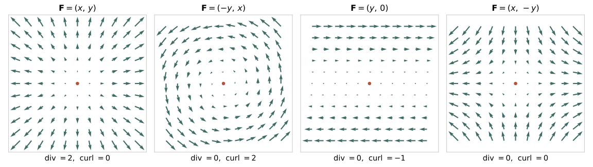
The figure shows four typical 2D fields. The first two are pure expansion and pure rotation. The third, a simple shear, contains both rotation and deformation. The fourth is pure deformation: its divergence and curl both vanish, yet it is clearly not a trivial field.

Formalism

Write $\mathbf{F} = (P, Q, R)^\top$ and use subscripts for partial derivatives, e.g. $P_y = \partial P / \partial y$. The Jacobian is

$$J = \begin{bmatrix} P_x & P_y & P_z \\ Q_x & Q_y & Q_z \\ R_x & R_y & R_z \end{bmatrix}.$$

Divergence is the trace of the Jacobian

$$\nabla\cdot\mathbf{F} = P_x + Q_y + R_z = \operatorname{tr} J .$$

Why the trace measures volume change. In time $dt$ the velocity field carries the point $\mathbf{x} + \mathbf{h}$ to $\mathbf{x} + \mathbf{h} + \mathbf{F}(\mathbf{x} + \mathbf{h})\,dt$. Relative to the parcel’s centre, a small offset $\mathbf{h}$ is mapped to

$$\mathbf{h} \mapsto (I + J\,dt)\,\mathbf{h} + o(\|\mathbf{h}\|) .$$

The volume of a small element scales by the determinant of this linear map. By the Leibniz formula, $\det(I + J\,dt)$ is a sum over permutations:

• the identity permutation gives the product of the diagonal, $\prod_i (1 + J_{ii}\,dt) = 1 + \operatorname{tr}J\,dt + O(dt^2)$;
• every other permutation contains at least two off-diagonal factors, each carrying a $dt$, so it contributes $O(dt^2)$.

Therefore

$$\det(I + J\,dt) = 1 + \operatorname{tr}J\,dt + O(dt^2), \qquad \frac{1}{V}\frac{dV}{dt} = \nabla\cdot\mathbf{F} .$$

Divergence is the instantaneous relative rate of change of local volume: positive means expansion, negative means compression, zero means no first-order change in volume. Zero divergence implies neither zero velocity nor an unchanged shape.

Two quantities are easy to confuse here. $\det J$ is the local volume scaling of a map itself; $\operatorname{tr}J$ is the rate of volume change caused by a velocity field. The short-time map $I + J\,dt$ connects them.

Curl comes from the antisymmetric part of the Jacobian

$$\nabla\times\mathbf{F} = \begin{bmatrix} R_y - Q_z \\ P_z - R_x \\ Q_x - P_y \end{bmatrix}.$$

Each component is the difference of a pair of mirror-image entries of the Jacobian, so curl depends only on the antisymmetric part $W = \frac12(J - J^\top)$.

Half the curl is the local angular velocity. Let $\boldsymbol{\omega} = \nabla\times\mathbf{F}$, with cross-product matrix

$$[\boldsymbol{\omega}]_\times = \begin{bmatrix} 0 & -\omega_3 & \omega_2 \\ \omega_3 & 0 & -\omega_1 \\ -\omega_2 & \omega_1 & 0 \end{bmatrix}, \qquad [\boldsymbol{\omega}]_\times \mathbf{h} = \boldsymbol{\omega} \times \mathbf{h} .$$

Writing out $J - J^\top$ entry by entry,

$$J - J^\top = \begin{bmatrix} 0 & P_y - Q_x & P_z - R_x \\ Q_x - P_y & 0 & Q_z - R_y \\ R_x - P_z & R_y - Q_z & 0 \end{bmatrix}.$$

Compare with $[\boldsymbol{\omega}]_\times$: at $(1,2)$, $-\omega_3 = P_y - Q_x$; at $(1,3)$, $\omega_2 = P_z - R_x$; at $(2,3)$, $-\omega_1 = Q_z - R_y$. They match exactly, so

$$J - J^\top = [\nabla\times\mathbf{F}]_\times , \qquad W\mathbf{h} = \tfrac12\,(\nabla\times\mathbf{F}) \times \mathbf{h} .$$

A rigid body spinning with angular velocity $\boldsymbol{\Omega}$ has velocity $\boldsymbol{\Omega} \times \mathbf{h}$. Comparing the two, the local rigid rotation of the parcel has angular velocity

$$\boldsymbol{\Omega} = \tfrac12\,\nabla\times\mathbf{F} .$$

A $3 \times 3$ antisymmetric matrix has exactly three independent entries, which is why it can be represented by an axial vector, and why curl is a vector only in three dimensions. In 2D the antisymmetric part has a single entry, and curl is the scalar $Q_x - P_y$, a rotation about the axis normal to the plane.

Example. $\mathbf{F} = (-2y, 2x, 0)^\top$ is a rigid rotation about the $z$-axis with angular velocity 2. Its divergence is 0 and its curl is $(0, 0, 4)^\top$, exactly twice the angular velocity.

The full decomposition of the Jacobian

Split the Jacobian into symmetric and antisymmetric parts, then remove the trace from the symmetric part:

$$J = \underbrace{\frac{\operatorname{tr}J}{3}\,I}_{\text{uniform expansion}} + \underbrace{\Big(\frac{J + J^\top}{2} - \frac{\operatorname{tr}J}{3}\,I\Big)}_{\text{symmetric traceless deformation}} + \underbrace{\frac{J - J^\top}{2}}_{\text{rotation}} .$$

The three parts have $1 + 5 + 3 = 9$ degrees of freedom, exactly the nine entries of the Jacobian. Divergence reads only the first part (one number) and curl only the third (three numbers); the five degrees of freedom of volume-preserving deformation in between are invisible to both.

Counterexample. $\mathbf{F} = (x, -y, 0)^\top$ has Jacobian $\operatorname{diag}(1, -1, 0)$. Its divergence and curl are both zero, yet it stretches along $x$ and squeezes along $y$. Divergence and curl at a point cannot recover the Jacobian there.

Simple shear. The field $\mathbf{F} = (y, 0)$ in the figure has Jacobian $\begin{bmatrix} 0 & 1 \\ 0 & 0 \end{bmatrix}$. Its symmetric part $\begin{bmatrix} 0 & 1/2 \\ 1/2 & 0 \end{bmatrix}$ is deformation, and its antisymmetric part $\begin{bmatrix} 0 & 1/2 \\ -1/2 & 0 \end{bmatrix}$ is a rotation with angular velocity $-1/2$ (clockwise); the 2D curl is $Q_x - P_y = -1$. A flow that looks like layers simply sliding past each other contains both rotation and deformation.

Integral forms: flux and circulation

Divergence and curl also have coordinate-free definitions.

Divergence is net outward flux per unit volume. Take a small cube of side $h$ centred at $\mathbf{x}$. The two faces normal to the $x$-axis contribute a net outward flux

$$\big[P(x + \tfrac{h}{2}) - P(x - \tfrac{h}{2})\big]\,h^2 \approx P_x\, h^3 ,$$

and the other two pairs of faces contribute likewise. Adding the three gives a net outward flux $\approx (P_x + Q_y + R_z)\,h^3$, so

$$\nabla\cdot\mathbf{F}(\mathbf{x}) = \lim_{V \to \mathbf{x}} \frac{1}{|V|}\oint_{\partial V} \mathbf{F}\cdot\mathbf{n}\, dS .$$

A component of curl is circulation per unit area. For a small surface $S$ through $\mathbf{x}$ with normal $\mathbf{n}$,

$$(\nabla\times\mathbf{F})\cdot\mathbf{n} = \lim_{S \to \mathbf{x}} \frac{1}{|S|}\oint_{\partial S} \mathbf{F}\cdot d\mathbf{r} ,$$

with the boundary oriented by the right-hand rule relative to $\mathbf{n}$.

Adding these local relations over a whole region, the contributions of neighbouring cells cancel in the interior and only the boundary survives. This gives the two integral theorems:

Theorem	Formula	Meaning
Divergence theorem	$\int_V \nabla\cdot\mathbf{F}\, dV = \oint_{\partial V} \mathbf{F}\cdot\mathbf{n}\, dS$	Total source inside equals net flux through the boundary
Stokes’ theorem	$\int_S (\nabla\times\mathbf{F})\cdot\mathbf{n}\, dS = \oint_{\partial S} \mathbf{F}\cdot d\mathbf{r}$	Total local circulation on the surface equals circulation around its edge

Both require a sufficiently smooth field, a sufficiently regular region and consistent orientation. Chapter 3 uses the divergence theorem to derive the Poisson equation.

The two zero identities

Gradient fields are curl-free: $\nabla\times(\nabla f) = 0$. The first component is $\partial_y\partial_z f - \partial_z\partial_y f$, which vanishes because mixed partials commute for twice continuously differentiable $f$; the other components are the same.

Curl fields are divergence-free: $\nabla\cdot(\nabla\times\mathbf{F}) = 0$. Expanding,

$$\partial_x(R_y - Q_z) + \partial_y(P_z - R_x) + \partial_z(Q_x - P_y) = 0 ,$$

where the six terms cancel in pairs, again because mixed partials commute.

Both identities need enough smoothness and cannot be applied blindly at singular points.

Does zero curl imply a potential? Only on a simply connected region. Consider, on $\mathbb{R}^2 \setminus \{0\}$,

$$\mathbf{F} = \frac{(-y,\; x)}{x^2 + y^2} .$$

A direct computation gives $Q_x = P_y = (y^2 - x^2)/(x^2 + y^2)^2$, so $Q_x - P_y = 0$ everywhere. Around the unit circle, however, $\mathbf{F}\cdot d\mathbf{r} = d\theta$ and the circulation is $2\pi \neq 0$. If $\mathbf{F} = \nabla\phi$, every closed loop would have zero circulation, so this field has no global potential. The obstruction is the hole at the origin.

Conventions

• $\nabla$ is a differential operator, not a numeric vector. The “dot” and “cross” notation is a mnemonic; on products the product rule still applies, e.g. $\nabla\cdot(\phi\mathbf{F}) = \nabla\phi\cdot\mathbf{F} + \phi\,\nabla\cdot\mathbf{F}$.
• The formulas in this chapter hold in Cartesian coordinates only. In cylindrical and spherical coordinates the basis vectors vary with position and extra scale-factor terms appear; the Cartesian formulas cannot be copied over.

In robotics

Optical-flow divergence and time to contact

When a drone or robot approaches a facing plane along its optical axis, the optical flow in the image radiates outward from one point, the focus of expansion (FOE). The divergence of that flow gives the time to contact (TTC) directly.

Let the camera move forward along its optical axis with speed $W$ towards a plane at depth $Z$. In the camera frame, scene points have velocity $(\dot{X}, \dot{Y}, \dot{Z}) = (0, 0, -W)$. With normalized image coordinates $x = X/Z$ and $y = Y/Z$, differentiating in time gives

$$\dot{x} = \frac{\dot{X}}{Z} - \frac{X\dot{Z}}{Z^2} = \frac{W}{Z}\,x , \qquad \dot{y} = \frac{W}{Z}\,y .$$

The flow $(\dot{x}, \dot{y}) = \frac{W}{Z}(x, y)$ is exactly the “source” field of the figure, with the FOE at the principal point. Its divergence is

$$\frac{\partial \dot{x}}{\partial x} + \frac{\partial \dot{y}}{\partial y} = \frac{2W}{Z} = \frac{2}{\tau}, \qquad \tau = \frac{Z}{W} .$$

Three properties of this result stand out:

• measuring the flow divergence yields the time to contact $\tau$ without knowing the depth $Z$ or the speed $W$ separately;
• in pixel coordinates $u = f x + c_x$ both the flow and the coordinates are scaled by $f$, so the divergence is unchanged and the focal length is not needed either;
• divergence measures expansion, and the third column of the projection Jacobian in Chapter 1 shows that motion along the optical axis is precisely what moves image points radially.

These properties are why flow divergence is widely used for obstacle avoidance and landing control on micro air vehicles, for example by holding the divergence constant to produce a smooth decelerating descent. The derivation above holds only for pure forward motion towards a facing plane; lateral translation, a slanted plane or rotation add further terms to the divergence, which must be compensated first.

The curl of optical flow corresponds to rotation about the optical axis. If the camera rotates about its optical axis with rate $\omega_z$, scene points move in the camera frame with velocity $(\omega_z Y, -\omega_z X, 0)$, the image flow is $(\omega_z y, -\omega_z x)$, and its 2D curl is $-2\omega_z$: twice the angular rate, with the sign opposite to the camera’s rotation. This matches the result that half the curl is the angular velocity.

Experiment

The first script computes, on a grid, the divergence and curl of the four fields in the figure and includes the plotting code.

import numpy as np
import matplotlib.pyplot as plt

x = np.linspace(-1, 1, 41)
y = np.linspace(-1, 1, 41)
X, Y = np.meshgrid(x, y)              # shape (ny, nx); X varies along axis=1

fields = {
    "source": (X, Y),
    "vortex": (-Y, X),
    "shear":  (Y, 0 * X),
    "strain": (X, -Y),
}

def div_curl(P, Q):
    dP_dy, dP_dx = np.gradient(P, y, x)
    dQ_dy, dQ_dx = np.gradient(Q, y, x)
    return dP_dx + dQ_dy, dQ_dx - dP_dy

for name, (P, Q) in fields.items():
    d, c = div_curl(P, Q)
    print(f"{name:7s} div = {round(d.mean(), 2) + 0.0:+.2f}   curl = {round(c.mean(), 2) + 0.0:+.2f}")
# source  div = +2.00   curl = +0.00
# vortex  div = +0.00   curl = +2.00
# shear   div = +0.00   curl = -1.00
# strain  div = +0.00   curl = +0.00

fig, axes = plt.subplots(1, 4, figsize=(12, 3.4))
s = slice(None, None, 4)
for ax, (name, (P, Q)) in zip(axes, fields.items()):
    ax.quiver(X[s, s], Y[s, s], P[s, s], Q[s, s])
    ax.set_title(name)
    ax.set_aspect("equal")
plt.show()

The second script synthesizes the flow of a camera approaching a plane, checks that its divergence equals $2/\tau$, and checks that rotation about the optical axis gives a curl of $-2\omega_z$.

import numpy as np

W, Z = 2.0, 10.0                      # approach at 2 m/s from 10 m: tau = 5 s
f = 400.0                             # focal length in pixels
px = np.linspace(-200, 200, 81)       # pixel coordinates relative to the principal point
U, V = np.meshgrid(px, px)
xn, yn = U / f, V / f                 # normalized coordinates

# pure forward motion: pixel flow = f * (W/Z) * (x, y)
flow_u, flow_v = f * xn * W / Z, f * yn * W / Z
div = np.gradient(flow_u, px, axis=1) + np.gradient(flow_v, px, axis=0)
print(div.mean(), 2 * W / Z, "tau =", 2 / div.mean())   # about 0.4 0.4 tau = 5.0 (up to rounding)

# rotation about the optical axis: pixel flow = f * omega * (y, -x)
omega = 0.3
rot_u, rot_v = f * omega * yn, -f * omega * xn
curl = np.gradient(rot_v, px, axis=1) - np.gradient(rot_u, px, axis=0)
print(curl.mean(), -2 * omega)                          # about -0.6 -0.6

References

1. Koenderink, J. J., & van Doorn, A. J. (1976). Local structure of movement parallax of the plane. Journal of the Optical Society of America, 66(7), 717–723.
2. Lee, D. N. (1976). A theory of visual control of braking based on information about time-to-collision. Perception, 5(4), 437–459.
3. Herissé, B., Hamel, T., Mahony, R., & Russotto, F.-X. (2012). Landing a VTOL unmanned aerial vehicle on a moving platform using optical flow. IEEE Transactions on Robotics, 28(1), 77–89.
4. Schey, H. M. (2005). Div, Grad, Curl, and All That (4th ed.). W. W. Norton.
5. OpenStax. Calculus Volume 3, Section 6.5: Divergence and Curl. https://openstax.org/books/calculus-volume-3/pages/6-5-divergence-and-curl
6. 3Blue1Brown. Divergence and curl: The language of Maxwell’s equations, fluid flow, and more. https://www.3blue1brown.com/lessons/divergence-and-curl/
7. MIT OpenCourseWare. 18.02SC Multivariable Calculus (Fall 2010), Unit 4: Triple integrals and surface integrals in 3-space (including the divergence theorem and Stokes’ theorem). https://ocw.mit.edu/courses/18-02sc-multivariable-calculus-fall-2010/